In the second part of this tutorial you will learn how to create sinusoidal flow profiles using JavaScript functions. To do this, you modify the script from the first part so that a sinusoidal profile is generated instead of a sawtooth profile. Before you start with this second part, you may want to read the first part of the tutorial here.
Important
For this tutorial you need the QmixElements version v20191121 or a newer version. If you are still using an older version, please update to the latest QmixElements version.
Preparation
Configure your system as described in the first part of the tutorial and then connect to your devices. If you do not have the appropriate devices, you are welcome to follow the tutorial with simulated devices. The QmixElements project with simulated devices and the script created in the first tutorial can be downloaded here.
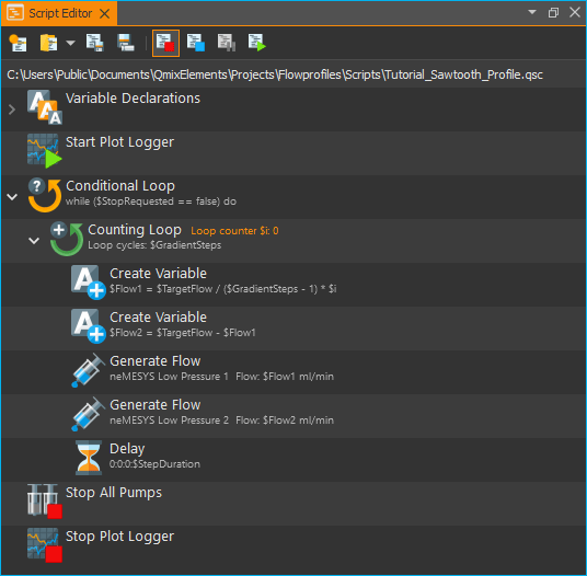
Now open the script Tutorial_Sawtooth_Profile.qsc that you created in the first part of the tutorial and save it under a new name. You should then see the following program in script editor.
Part 2 – Script for generating a sinusoidal profile
The goal of this script is to generate a flow profile in the form of a sine wave from 0 to the defined target flow rate with one pump and to supplement the flow of the first pump with the second pump in such a way that the sum of the two flows results in a constant flow with a defined flow rate.
To generate the profile, the flow rate of the pump must be changed step by step so that a sinusoidal profile is created over time. The number of steps for generating the sine profile, i.e. the resolution, should be set to 100 steps for one sine. In the previous sawtooth script you had set the number of steps to 20. Therefore change the value of the variable $GradientSteps to 100.
Adjusting the resolution (number of steps) for a sine profile
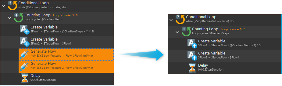
Now delete the two Generate Flow functions as shown in the figure below. To do this, select both functions and then delete them using the context menu (right mouse button) or by pressing the Delete key.
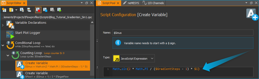
Now insert a new variable before the two existing variables in the counting loop. Name the variable $Sinus and select JavaScript Expression in the Type field.

The $Sine variable is used to store the calculation of the sine value for further processing. To calculate the sine value, use the JavaScript function Math.sin() together with the constant Math.PI. Enter the following into the input field for the JavaScript expression:
Math.sin(2 * Math.PI / ($GradientSteps – 1) * $i)
The loop counter $i runs from 0 to the number of $GradientSteps – 1. To calculate the current sine value, the period 2π is divided by the number of steps – 1 and then multiplied by the current step $i.
To check the calculated value of the $Sine variable, you can display its value in the graphical logger. To do this, you have already created the virtual I/O channel Script Value 1 in the first part of the tutorial and added it to the graphical logger. Now insert the function Write Device Property ❶ into the script. Then configure the function as shown in the figure below.
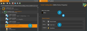
In the field Value to be written ❷ enter the variable name $Sinus. In the Device Property area ❸ select in the Devicefield the virtual channel Script Value 1. In the Property field select the property ActualValue. You can now read the function as follows:
Write the value of the variable $Sinus into the property ActualValue of the virtual channel Script Value 1.
Now delete all data from the graphical logger and activate automatic scaling. Now start your script. If you have entered everything correctly, you should see how the following sine function is generated in the graphical logger:
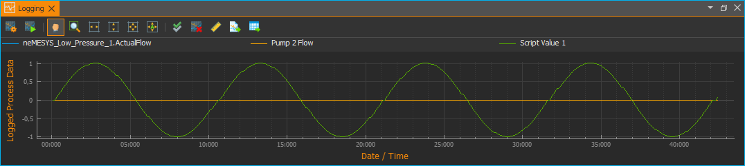
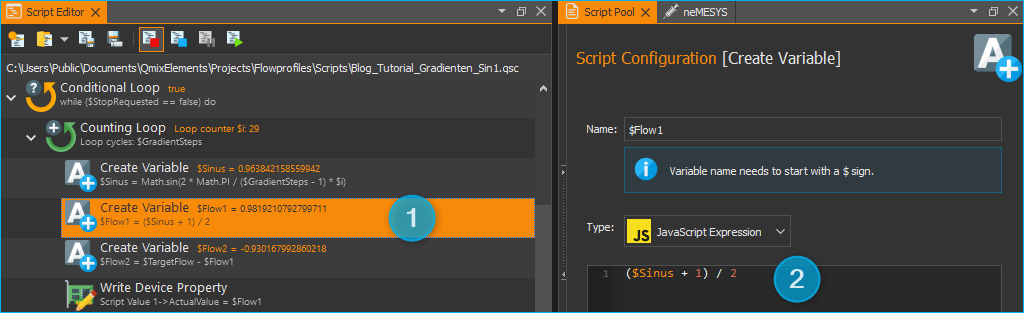
The sine oscillates between 1 and -1 as expected. For the sinusoidal flow profile to be generated, the flow rate should oscillate between 0 and the target flow rate. In a first step, the sine value should be adjusted so that it oscillates between 0 and 1. You can achieve this by shifting the sine on the Y-axis upwards by 1 and then halve the amplitude. To store the new value, we use the existing variable $Flow1 ❶. This can now be calculated like this:
❷ $Flow1 = ($Sine + 1) / 2
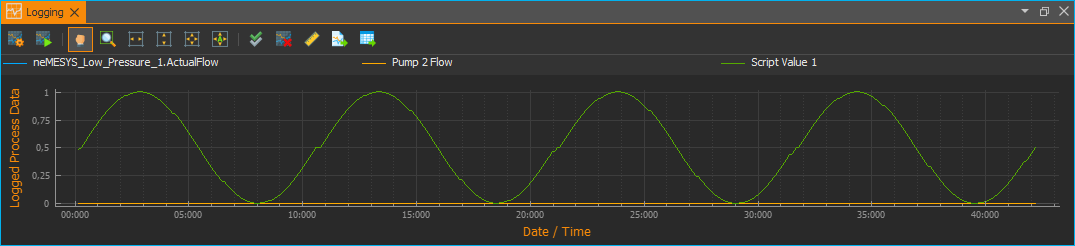
Now change the Write Device Property function so that the value of the variable $Flow1 is displayed instead of the value of the variable $Sine. Then delete the graphical logger and reactivate automatic scaling. You should now see the following function in the graphic logger – a sine function oscillating between 0 and 1:
To make the sine oscillate between 0 and the target flow rate, you now only have to multiply by the target flow rate $TargetFlow. Extend the calculation of the variable $Flow1 by this step:
$Flow1 = ($Sine + 1) / 2 * $TargetFlow
The flow rate $Flow1 will now oscillate sinusoidally between 0 and the target flow rate. The flow rate $Flow2 of the second pump should complement the first flow rate in such a way that a constant flow with a constant flow rate $TargetFlow is created. You can therefore calculate the flow rate of the second pump in the variable $Flow2 as follows:
$Flow2 = $TargetFlow – $Flow1
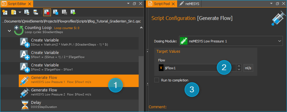
Now insert two Generate Flow functions in front of the Write Device Property function and then delete the Write Device Property function as it is no longer needed.
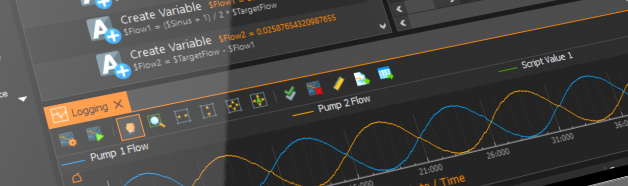
The script should now look like the figure below ❶. Configure the two Generate Flow functions to start the first pump at flow rate $Flow1 ❷ and the second pump at flow rate $Flow2 (see figure below). Make sure that the Run to completion option ❸ is disabled.
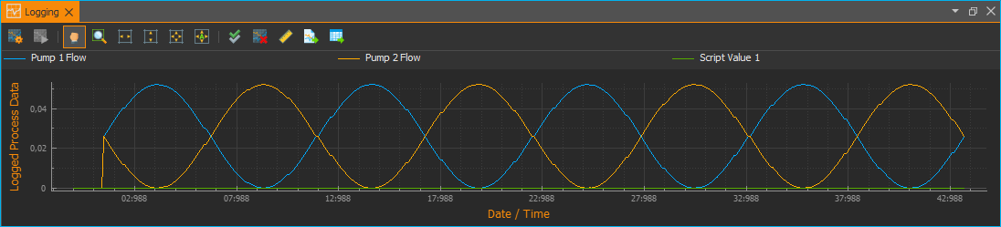
Now delete all data from the graphical logger again and activate automatic scaling. Before starting the script, check that the syringes of both pumps are filled. Then start your script. If you have entered everything correctly, you should see how the following flow profiles are generated in the graphical logger:
You have now learned the basics of how to use JavaScript in the script functions – e.g. to perform mathematical calculations. Apply what you have learned, for example by programming a script that generates two sinusoidal flows, where the sine of the second flow has twice the period of the sine of the first flow. Use the graphical logger to check the results.
In the third part of the tutorial you will learn how to add an initialization routine to the script, how to wind up the syringes and get tips on how to improve the readability of your script and how to document your script.
The QmixElements project with simulated devices and the scripts created in the first and second part of the tutorial can be downloaded here.