The QmixElements software has a powerful script system to automate processes and procedures quickly and easily. This tutorial will give you an insight and many useful hints on some of the advanced features of QmixElements. Techniques, such as the use of variables, the use of JavaScript and the use of virtual channels for recording values in the graphical logger.
In this tutorial, you will create two scripts that generate flow gradients or flow profiles based on mathematical functions.
Preparation
Before you can start programming the scripts, you must configure your system. If you do not have the appropriate devices, you are welcome to follow the tutorial with simulated devices. You can download the QmixElements project with simulated devices and the script created in the tutorial here.
Important
For this tutorial you need the QmixElements version v20191121 or a newer version. If you are still using an older version, please update to the latest QmixElements version.
Latest QmixElements Version
For this tutorial we used two neMESYS low pressure syringe pumps with 5 ml glass syringes ❶. You can do this tutorial with other neMESYS syringe pumps or syringes, but you may have to adjust the flow rates. To switch the valves automatically during the generation of the flow profiles, activate the valve automation for both pumps ❷. Please configure ml/min ❸ as the unit for the flow rate.
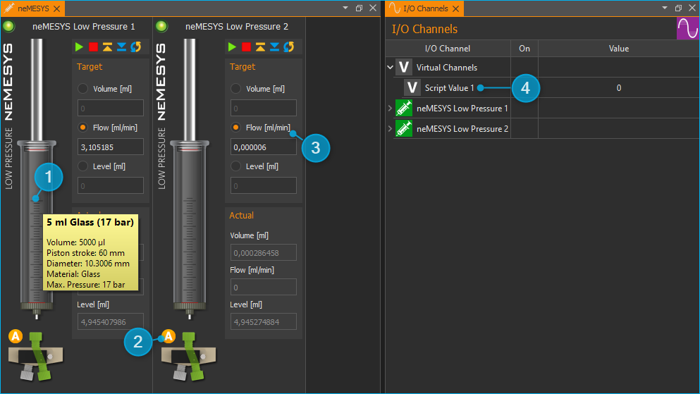
To visualize calculated values from the script graphically, create a virtual channel ❹in the list of I/O channels. A virtual channel is an I/O channel that can be used for entering and outputting values.
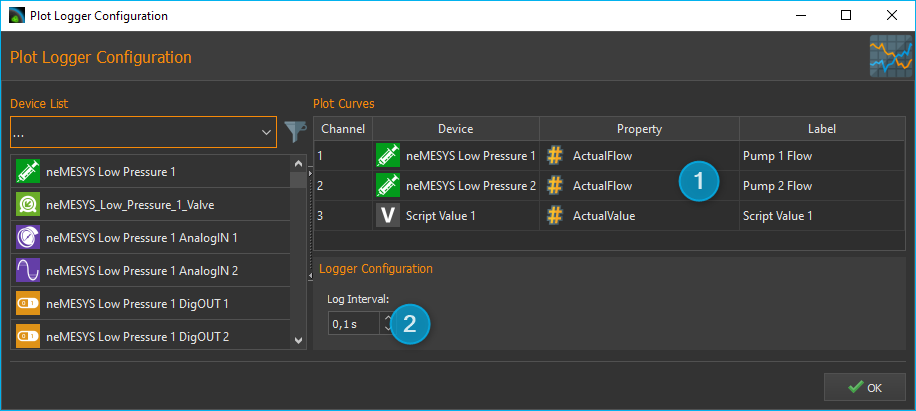
To record and visualize the generated flow profiles graphically in real time, use the graphical logger and configure it according to the figure below. The current flow rate of both pumps should be displayed as well as the current value of the virtual channel ❶. As Log Interval❷ set a value of 0.1 seconds. Now you can start programming the first script.
Part 1 – Script for generating a sawtooth profile
The aim of this script is to generate a flow profile in the form of a sawtooth with one pump and to supplement the flow of the first pump with the second pump so that the sum of the two flows leads to a constant flow with a defined flow rate but with a mixing ratio that changes over time.
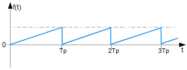
The sawtooth is generated by increasing the flow rate stepwise in a fixed interval from 0 to the desired target flow rate. The following parameters can be identified for the script:
- Number of steps for a single sawtooth ($GradientSteps)
- Duration of a step in milliseconds ($StepDuration)
- Target flow rate ($TargetFlow)
You create three variables for these parameters in your script. So you can change the parameters later quickly and easily in one place, without having to navigate through the complete script all the time. For each variable you assign a meaningful and unique name.
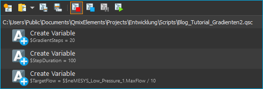
For the gradient, use 20 steps ($GradientSteps = 20) with a duration of 100 milliseconds each ($StepDuration = 100). The resolution of 100 ms is a reasonably fast time base for many applications. You can change these values later at any time. You can enter a fixed value for the target flow rate, or you can calculate the target flow rate based on the maximum flow rate of the first pump. To do this, you can insert the device property (Insert device property) for the maximum flow rate of the pump into the JavaScript field and use it for calculations. In this example we want to dose with one tenth of the maximum flow rate and therefore simply divide it by 10. You can also use other values or your own calculations:
$TargetFlow = $neMESYS_Low_Pressure_1.MaxFlow / 10
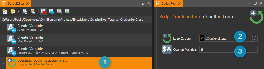
To create a single sawtooth, you now need a Counting Loop ❶. Two parameters can be configured for a counting loop: the number of Loop Cycles ❷ and the name of the variable (Counter Variable) in which the counter value for the current loop cycle is stored ❸. The input field for the loop cycles ❷ is marked with an orange V, i.e. you can use variables in this input field. At this point you can simply enter the previously defined variable $GradientSteps.
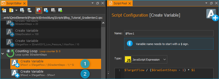
Within the loop you can now calculate the flow rate for the first pump and save it in a variable. The loop counter $i takes the values 0 – 19 for the 20 loop passes. You can therefore calculate the flow rate with the following formula:
❶ $Flow1 = $TargetFlow / ($GradientSteps – 1) * $i
I.e. the flow rate is 0 in the first loop pass and reaches the value $TargetFlow in the last loop pass. The sum of the flow rates of both pumps should give the value $TargetFlow. Therefore, in a second variable, you can calculate the flow rate of the second pump as follows:
❷ $Flow2 = $TargetFlow – $Flow1
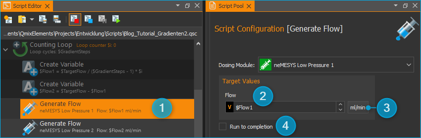
You can now use these two values to start the dosing of the two pumps with the function Generate Flow ❶. To configure the Generate Flow function, simply select the appropriate pump and enter the calculated value $Flow1 or $Flow2 in the Flow field ❷. It is important that the unit for the flow rate is set to the same value as configured for the pump – in this case ml/min ❸. You have to deactivate the Run to completition checkbox ❹. If this field is active, the next function will not be started until the pump has finished dosing. In the case of the Generate Flow function, this would be when the pump is fully wound or drained. Since this is not desired here, but the script is to be continued immediately, deactivate the field.
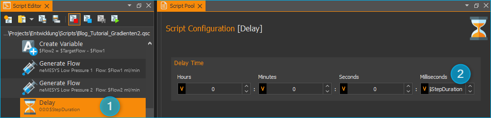
To achieve the desired step duration for each loop cycle, add a Delayfunction ❶ as the last function in the loop. You can directly enter the variable $StepDuration in the configuration area of the function in the input field Milliseconds ❷. The Delay function delays the further execution of the script for the configured time period.
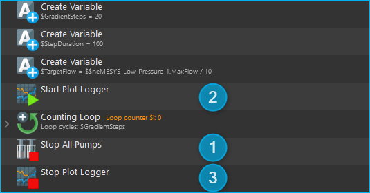
At the end of your short script, now add the Stop All Pumps ❶ to stop all pumps. To synchronize the recording of the flow rates in the graphical logger with the script flow, add the function to start the logger (Start Plot Logger) ❷ before the counting loop and the function to stop the recording (Stop Plot Logger) ❸ at the end of the script.
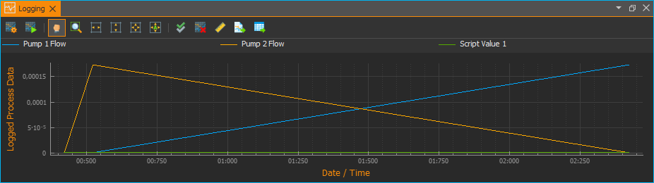
When your syringes are completely filled, you can now start the first test run. If the script has run without errors, you should see the following graphs in the graphical logger.
In the next step, extend the script to repeat the generation of the sawtooth cyclically until the user presses the Request Script Stop ❶ button. To do this, insert a Conditional Loop ❷ in front of the sawtooth loop. In the configuration area of the function, switch to the JavaScript area ❸ and enter the following condition:
❹ $StopRequested == false
This means that this loop is repeated continuously as long as the condition is fulfilled, i.e. as long as the global variable $StopRequested has the value false. The variable $StopRequested is a global script variable that is always present. After starting the script this variable always has the value false. Only when the user presses the button Request Script Stop ❶, the value of the variable is set to true.
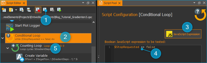
Now you can insert the sawtooth loop into the conditional loop. Click on the Counting Loop ❺ and drag it to the Conditional Loop ❷. The counting loop is then inserted into the conditional loop. Now restart the script. The generation of the sawtooth is now repeated until you press the button Request Script Stop ❶.
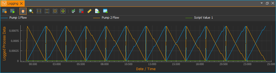
After a few cycles, press the Request Script Stop ❶ button to end the script. If the script has run without errors, you should see the following graphs in the graphical logger.
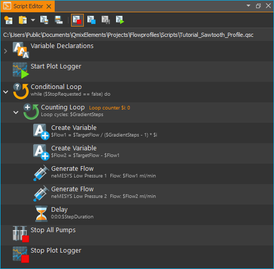
Your flow profile script is almost finished. To improve the clarity, you can combine the variables you declared at the beginning of the script in a variable group (Variable Declarations). Insert a Variable Declarations function as the first function in the script. Then select all variables. Click on the first Create Variable function and then click on the last Create Variable function while holding down the Shift key – just as you would select several files in your file explorer.
Afterwards you can move all marked variables with the mouse into the variable group. With this you have grouped the variables and improved the clarity and readability of the script. In addition, it is now easier to move this group of variables to another position. Your script should now look like this:
In the second part of the tutorial you will learn how to modify the script so that sinusoidal flow profiles can be generated with the help of JavaScript functions. You will also learn how to add an initialization routine to the script that pulls up the syringes and how to record calculated values using virtual I/O channels in the graphical logger. Finally, you will receive tips on how to improve the readability of your script and document your script.
The QmixElements project with simulated devices and the script created in the tutorial can be downloaded here.